In this post you’ll learn to unfold a list from a value with a recursion wrapper called LIST.UNFOLD.

INTRODUCTION

In Excel as in many other languages, we can use REDUCE to reduce (or fold) a list into a single value. We iterate over the list, and at each element apply a function. The result of that function becomes what’s known as an accumulator. This accumulator created from applying the function to one element is passed as an argument to the same function when it is applied to the next element. This continues until the last element of the list is reached, at which point the accumulator becomes the result.

So, with REDUCE, we can create a single value from a list and a function.

In some languages this operation is known as “folding”. In fact, I talked about that in an earlier post. It turns out that in several functional programming languages have built-in capability to do the opposite of the reduce (or fold) operation.

Let’s look at List.unfold from F#. Here’s the example from the documentation:

|> List.unfold (fun state -> if state > 100 then None else Some (state, state * 2))

Both Some and None are part of what’s known as an Option type in F#. They are used to safely handle values that might or might not exist. When the if statement returns true, i.e. when state is greater than 100, the return of None is an error-safe way to indicate that there are no more values to add to the list. This is essentially the exit condition to tell List.unfold to stop. If state is less than or equal to 100, Some (state, state * 2) creates a tuple whose first element is the next element to be added to the list. The second element is the new value of state to pass to the next iteration of the generator function. So, this is a concise way of using recursion to generate a list and one of the many reasons why F# is a great language!

Reading this you may be thinking… hey, is that why we have List.Generate in Power Query?

Yes. Yes, it is.

In fact, my observation is that List.Generate encapsulates the functionality of List.unfold and adds additional functionality to handle common data mashup use cases that might be needed in the realms of Excel, Power BI et al.

Anyway, we’re getting off track! Let’s look at LIST.UNFOLD as an Excel LAMBDA function!

LIST.UNFOLD

Here’s the code for LIST.UNFOLD:

LIST.UNFOLD = LAMBDA(generator_function, 
    LAMBDA(value,
        LET(
            _result, generator_function(value),
            IF(ISNA(@TAKE(_result,-1, 1)), value, LIST.UNFOLD(generator_function)(_result))
        )
    )
);

Looks simple, right? And it is! I’ll break it down for you in a minute, but let’s talk about the signature. There are two required (and curried) parameters. The reason for that will become clear shortly.

  1. generator_function – this is the function that will take the current state of the list and produce a new value to be added. This function can be very simple or incredibly complex. The requirement placed on this function is that it has one parameter. There is no requirement on the type of that parameter.
  2. value – this is the current state of the list. When we call LIST.UNFOLD, we’ll give this inner lambda a seed value to get started on, and as the function recurses, the list being created will be passed into this parameter.

Here’s an example of how LIST.UNFOLD works:

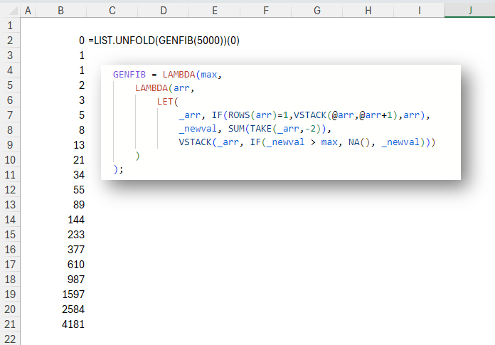
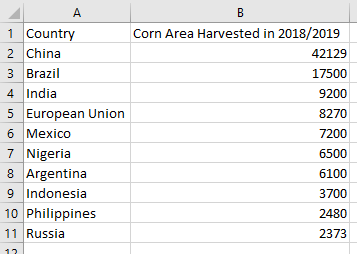
GENFIB is a general implementation of a Fibonacci-like sequence. This function calculates the new value as the sum of the previous two values. It then stacks the new value underneath the previous values. Here’s the code for GENFIB:

GENFIB = LAMBDA(max,
    LAMBDA(arr, 
        LET(
            _arr, IF(ROWS(arr)=1,VSTACK(@arr,@arr+1),arr),
            _newval, SUM(TAKE(_arr,-2)), 
            VSTACK(_arr, IF(_newval > max, NA(), _newval)))
    )
);

The important thing here is that we can configure the exit condition by passing the first parameter as the value which will serve as an exit condition for the function. So this:

GENFIB(5000)

Returns this:

    LAMBDA(arr, 
        LET(
            _arr, IF(ROWS(arr)=1,VSTACK(@arr,@arr+1),arr),
            _newval, SUM(TAKE(_arr,-2)), 
            VSTACK(_arr, IF(_newval > 5000, NA(), _newval)))
    )

Now we can see that if the _newval (state) is greater than 5000, the function will stack NA() to the bottom of the list. This is a design decision I’ve made for LIST.UNFOLD. When LIST.UNFOLD encounters an NA() at the bottom of the list, it will stop. So any function passed to LIST.UNFOLD must use this fact to control the exit condition.

One thing to note about GENFIB itself is that it is not a recursive function. All it does is calculate one value. The recursion is handled by LIST.UNFOLD. This is a way to remove the difficult part of the programming from the logic of the sequence and re-use it whenever it’s needed.

Without further ado, let’s take a close look at how LIST.UNFOLD works!

BREAKDOWN

For reference, here’s the code for LIST.UNFOLD again. I’ve included the code for GENFIB as it may be helpful in the following explanation.

LIST.UNFOLD = LAMBDA(generator_function, 
    LAMBDA(value,
        LET(
            _result, generator_function(value),
            IF(ISNA(@TAKE(_result,-1, 1)), value, LIST.UNFOLD(generator_function)(_result))
        )
    )
);

GENFIB = LAMBDA(max,
    LAMBDA(arr, 
        LET(
            _arr, IF(ROWS(arr)=1,VSTACK(@arr,@arr+1),arr),
            _newval, SUM(TAKE(_arr,-2)), 
            VSTACK(_arr, IF(_newval > max, NA(), _newval)))
    )
);

So, we pass a generator_function into the outer lambda of LIST.UNFOLD. An example is GENFIB(5000) which returns the function discussed above:

=LIST.UNFOLD(GENFIB(5000))

That returns this inner function:

    LAMBDA(value,
        LET(
            _result, generator_function(value),
            IF(ISNA(@TAKE(_result,-1, 1)), value, LIST.UNFOLD(generator_function)(_result))
        )
    )

Where generator_function is:

    LAMBDA(arr, 
        LET(
            _arr, IF(ROWS(arr)=1,VSTACK(@arr,@arr+1),arr),
            _newval, SUM(TAKE(_arr,-2)), 
            VSTACK(_arr, IF(_newval > 5000, NA(), _newval)))
    )

When you expand all of this, that small line has actually created this function!

UNFOLD.GENFIB5000 = 
    LAMBDA(value,
            LET(
                generator_function, 
                    LAMBDA(arr, 
                        LET(
                            _arr, IF(ROWS(arr)=1,VSTACK(@arr,@arr+1),arr),
                            _newval, SUM(TAKE(_arr,-2)), 
                            VSTACK(_arr, IF(_newval > 5000, NA(), _newval)))
                    ),
                _result, generator_function(value),
                IF(ISNA(@TAKE(_result,-1, 1)), value, LIST.UNFOLD(generator_function)(_result))
            )
        );

Which is part of the reason I wanted to put the recursion logic inside LIST.UNFOLD. Anyway, let’s get back on track. Here’s LIST.UNFOLD again.

LIST.UNFOLD = LAMBDA(generator_function, 
    LAMBDA(value,
        LET(
            _result, generator_function(value),
            IF(ISNA(@TAKE(_result,-1, 1)), value, LIST.UNFOLD(generator_function)(_result))
        )
    )
);

_result is the result of whatever generator_function produces when we give it value.

An example:

=LIST.UNFOLD(GENFIB(5000))(0)

This function passes 0 into the generator_function GENFIB(5000).

    LAMBDA(arr, 
        LET(
            _arr, IF(ROWS(arr)=1,VSTACK(@arr,@arr+1),arr),
            _newval, SUM(TAKE(_arr,-2)), 
            VSTACK(_arr, IF(_newval > 5000, NA(), _newval)))
    )

So 0 is arr. And since ROWS(0)=1, this GENFIB function assigns VSTACK(0, 0+1) to _arr. This is important because a Fibonacci-like calculation requires two values to calculate the next value. The design choice here is to say if this function has only been given one value, then we’ll just put the next integer after it and continue as if there were two values in the array originally.
_newval is then the sum of those two values. Finally, check if _newval is greater than 5000 and if it isn’t, return _arr with _newval stacked underneath.
This return value is, as mentioned, assigned to _result in LIST.UNFOLD:

LIST.UNFOLD = LAMBDA(generator_function, 
    LAMBDA(value,
        LET(
            _result, generator_function(value),
            IF(ISNA(@TAKE(_result,-1, 1)), value, LIST.UNFOLD(generator_function)(_result))
        )
    )
);

Passing 0 to value as we did means that _result will be {0; 1; 1} after the first iteration.

The next line of LIST.UNFOLD first checks if the last row in _result is NA(). If it is, LIST.UNFOLD exits and returns value (i.e. the state of the list after the previous iteration). If the value of the last row is not NA(), LIST.UNFOLD is called again, but this time _result is the new argument to value.
When value={0; 1; 1} in GENFIB, ROWS({0; 1; 1})=3, so _arr=arr and _newval=SUM(TAKE({0; 1; 1},-2))=SUM({1; 1})=2. Further, _newval is not greater than 5000, so the return value of the generator function is now VSTACK({0; 1; 1}, 2)={0; 1; 1; 2}, which becomes _result in UNFOLD.LIST, and so on and so forth until the exit condition is met!

The recursion, which is fairly standard behavior across the family of functions that produce sequences, is always handled in the same way, and so has been abstracted into the LIST.UNFOLD function. The real logic of what the syntax is is embedded in the generator function, which as I mentioned before, can be as simple or as complex as you like. Here are a few examples:

GEOMETRIC = LAMBDA(common_ratio, break_at, 
    LAMBDA(x, 
        LET(
            _newval, @TAKE(x,-1)*common_ratio, 
            VSTACK(x, IF(OR(AND(common_ratio<1,_newval<break_at),
                            AND(common_ratio>=1,_newval>break_at)), NA(), _newval))))
);

POWERSEQ = LAMBDA(power,ceiling,
    LAMBDA(x, LET(_newval, @TAKE(x,-1)^power, VSTACK(x,IF(_newval > ceiling, NA(), _newval))))
);

GENFIB = LAMBDA(max,
    LAMBDA(arr, 
        LET(
            _arr, IF(ROWS(arr)=1,VSTACK(@arr,@arr+1),arr),
            _newval, SUM(TAKE(_arr,-2)), 
            VSTACK(_arr, IF(_newval > max, NA(), _newval)))
    )
);

CATALAN =LAMBDA(max, mode, 
    LAMBDA(
        arr, 
        LET(
            _n, TAKE(arr,-1,-1), 
            _Cn, TAKE(arr,-1,1), 
            _newVal, _Cn * 2 * (2*_n + 1) / (_n + 2),
            VSTACK(arr, IF(
                IF(mode=0,_newVal,_n+2) > max
                , NA(), HSTACK(_newVal, _n + 1)))
        )
    )
);

These are somewhat trivial examples since, according to my 8-step process for writing recursive functions in Excel, they probably aren’t necessary.

However, I’d just like to remind you that recursion is either necessary for the program or for the programmer. If it makes the programming easier to understand, then use it!

SUMMARY

In this post we saw how to unfold a list with this new function – LIST.UNFOLD.

LIST.UNFOLD is a recursion wrapper for the family of functions that produce complex sequences. Like List.Generate in Power Query, and List.unfold in F#, we can pass a generator function to LIST.UNFOLD along with a seed value, to create a new list, making it equivalent to the reverse of REDUCE!

I hope you enjoyed reading about it and that it sparked some ideas. Let me know in the comments if you have any questions!

=LAMBDA(
    array_a,
    array_b,
    keep_duplicates,
    LET(
        arr,
        MAKEARRAY(
            ROWS(array_a)+ROWS(array_b),
            1,
            LAMBDA(r,
                   c,
                   IF(r<=ROWS(array_a),
                      INDEX(array_a,r),
                      INDEX(array_b,r-ROWS(array_a))
					  )
				   )
			     ),
        IF(keep_duplicates,arr,UNIQUE(arr))
		)
		)

You may have found yourself wanting to join two arrays together in Excel. This function will quickly append and optionally deduplicate two single-column arrays or ranges of data. This is done with the LAMBDA shown above, which you can define in Excel’s Name Manager with the name ARRAYUNION.

It accepts 3 arguments:

  1. array_a – a single-column array or range
  2. array_b – a single-column array or range
  3. keep_duplicates – a TRUE/FALSE value indicating whether to keep or remove duplicate values after appending array_b to array_a

It couldn’t be simpler to use:


The approach uses MAKEARRAY to create an array that has ROWS(array_a)+ROWS(array_b) rows and one column.

The elements of the array to be made are provided by the LAMBDA shown starting on line 10.

The first two arguments of that LAMBDA are r and c. Within the MAKEARRAY function, these represent row and column positions in the array being made.

Here we are saying if the row of the new array is less than or equal to the number of rows in array_a, then populate that row with the value from the same position in array_a (as retrieved by the INDEX function).

If the row of the new array is greater than the number of rows in array_a, then we will populate it with a value from array_b.

Let ‘arr’ be the array created by MAKEARRAY as described above. Then, if keep_duplicates is TRUE, return ‘arr’ unmodified. Otherwise, apply the UNIQUE function to ‘arr’ and return the result of that function call. This has the effect of removing duplicates from the joined arrays. This can be particularly useful if you have two lists of people on different sheets and you think there might be some people in both lists.

Or perhaps you have two reports with lists of products your company sells and you want to quickly create a combined report or check that the right products are included.

The gist for this lambda function can be found here.

If you sometimes need to quickly put some Excel data into a SQL table or use the data in a CTE, you may have found yourself doing something like this:

Here’s a LAMBDA I’ve called SQLVALUES:

=LAMBDA(t,LET(d,IFS(ISTEXT(t),”‘”&SUBSTITUTE(t,”‘”,”””)&”‘”,ISBLANK(t),”NULL”,LEFT(MAP(t,LAMBDA(x,CELL(“format”,x))),1)=”D”,TEXT(t,”‘YYYY-MM-DD HH:mm:ss'”),TRUE,t),”(“&TEXTJOIN(“,”,FALSE,d)&”)”))

This will:

  1. Wrap the tuple in parentheses
  2. Wrap text and dates in single-quotes
  3. Replace embedded single-quotes with escaped single-quotes
  4. Separate the columns with commas
  5. Format date-formatted cells as YYYY-MM-DD HH:mm:ss

If we’re inserting multiple values and our SQL database supports a list of tuples, we can also do this:

=LET(arr,A2:C6,BYROW(arr,SQLVALUES)&IF(LASTROW(arr),”;”,”,”))

Which is saying “Apply the SQLVALUES lambda to each row in arr. If the row of arr is the last row, put a semi-colon after it. Otherwise, put a comma after the row”.

LASTROW just takes an array and returns an array of TRUE/FALSE the same size as array. Here’s the LAMBDA for LASTROW:

=LAMBDA(d,ROW(d)=(ROWS(d)+MIN(ROW(d))-1))

You can now paste the data from the spreadsheet directly into your SQL editor.

I’m sure SQLVALUES is not perfect. I suspect there are edge cases it won’t cover, but hopefully it demonstrates a way to shortcut a task using array formulas and LAMBDA.

Do you have any suggestions for improvement to the SQLVALUES LAMBDA?


=LAMBDA(rng,vertical,LET(chars,MID(rng,SEQUENCE(LEN(rng)),1),IF(vertical,chars,TRANSPOSE(chars))))

This LAMBDA function takes two arguments:

  1. rng – a cell containing a text string
  2. vertical – TRUE/FALSE. If TRUE, the LAMBDA will return a vertical array of the characters in rng. If FALSE, the LAMBDA will return a horizontal array of the characters in rng

In my file, I have named this LAMBDA “CHARACTERS”. You can of course call it whatever you want.


So what?

This is useful, because it simplifies things when we want to extract all the numbers or text from a character string.


To get all the numbers in a horizontal array:

=LET(c,CHARACTERS($A$1,FALSE),nums,INT(c),FILTER(nums,NOT(ISERR(nums))))

To join the numbers from the array as a single integer:

=INT(CONCAT(LET(c,CHARACTERS($A$1,FALSE),nums,INT(c),FILTER(nums,NOT(ISERR(nums))))))

To get all the non-numbers in a horizontal array:

=LET(c,CHARACTERS($A$1,FALSE),nums,INT(c),FILTER(c,ISERR(nums)))

To get all the non-numbers as a single string:

=CONCAT(LET(c,CHARACTERS($A$1,FALSE),nums,INT(c),FILTER(c,ISERR(nums))))

Of course there are many other uses for this array of characters. We can test for a specific character in the array, or filter out specific sets of characters, or use it in a MAKEARRAY.

The CHARACTERS LAMBDA works principally because of this:

=MID(A1,SEQUENCE(LEN(A1),1)

This is simple but very powerful. SEQUENCE(LEN(A1) gives us a sequence of integers from 1 to the length of the string in A1. By passing this as the second parameter of MID, which is the “start”, and passing 1 as the third parameter, which says “get one character”, we are essentially applying the MID function as many times as there are numbers returned by SEQUENCE, and each of those times it’s applied, it is using one of the numbers in SEQUENCE. So, it’s the same as this:

The rest of the LAMBDA function is just deciding whether to return that array vertically or horizontally, by using the TRANSPOSE function.

In case it’s of use, here is a LAMBDA to get the numbers (you will also need the CHARACTERS LAMBDA defined above). I have called this GETNUMBERS.

=LAMBDA(rng,vertical,LET(c,CHARACTERS(rng,vertical),nums,INT(c),FILTER(nums,NOT(ISERR(nums)))))

And here’s one to get non-numbers, which I’ve called GETNONNUMBERS

=LAMBDA(rng,vertical,LET(c,CHARACTERS(rng,vertical),nums,INT(c),FILTER(c,ISERR(nums))))

If you want to quickly get all rows which don’t have any blanks in any columns, you can combine FILTER, BYROW and AND, like this:

=FILTER(range,BYROW(range,LAMBDA(r,AND(r<>””))))

Here, I’ve defined a LAMBDA function, which is really just a way of applying some logic (in the second parameter) to some data (in the first parameter). I have “r” as the name for my data.

By passing that LAMBDA as the second parameter of BYROW, I’m telling Excel that “r” represents a row of “range” and that I want the function AND(r <> “”) to be applied to that row.

That AND function will check if each column in the row is not empty. If they’re all not empty, it will be TRUE. If any column in that row is empty, it will be FALSE. So, BYROW does this for each row in the range and returns a 1-column array of TRUE/FALSE that has the same number of rows as “range”. I then use that TRUE/FALSE array as the “include” parameter of the FILTER function.

So, for the data in “range”, check if the cells in each row are all non-empty. If they are, then include the row. Otherwise, exclude it.

Where I’ve written “range” above, you would need to select exactly the same cells in both places. So, it may be easier to use LET to only have to select those cells once. Like this:

=LET(rng,A2:E12,FILTER(rng,BYROW(rng,LAMBDA(r,AND(r<>””)))))

LET allows you to give names to functions or ranges so you can re-use the name in several places in a formula instead of having to enter that function or range multiple times.

Further to all this, I think I’ll probably use this kind of thing again, so I can wrap the entire function in a LAMBDA function of its own and define it in the Name Manager. I’ve called it NONEMPTYROWS.

This is the LAMBDA called NONEMPTYROWS:

=LAMBDA(rng,FILTER(rng,BYROW(rng,LAMBDA(r,AND(r<>””)))))

If you wanted to switch this around to return only those rows that have a blank in any column, you would replace the AND(r<>””) with OR(r=””).

I downloaded some data from the USDA FAS custom query builder. The file contains the area harvested of corn in many harvest years for non-US countries.

I want to calculate the % of non-US corn area that each country represents in the latest two full harvest years and then calculate the change in percentage points between those two years. The downloaded data looks like this:

I’m going to use the harvest years “2017/2018” and “2018/2019”.  The first thing I’ve done is format the data as a table, by selecting anywhere in the data and pressing Ctrl+T, then I’ve given the table the name “corn_data” in the Table Name box in the Properties group on the Design tab in the Table Tools group on the ribbon.

The formatted table looks like this:

So, I said I want to calculate the % of non-US corn area that each country represents in the latest two full harvest years and then calculate the change in percentage points between those two years.

I can create a pivot table that looks like this:

To do that, I’ve put Area Harvested in the values area of the pivot table and changed the “Show values as” to “% of Column Total”.

I want to calculate for each row the difference for between the percentage for 2017/2018 and 2018/2019. Unfortunately, because I’ve already used “Show values as” to calculate the “% of Column Total”, I can’t use “Show values as” again to calculate the difference between the percentages!

I’ll probably have to put a simple formula in the next column, like this:

Simple enough, but not very flexible. If the pivot table changes shape (I add more columns), or I add too many filters, the formula will quickly get messed up and I’ll have to tweak it to keep it working.

Luckily, there’s a way to do both using PowerPivot. To get started, I’m going to add my formatted Table to the PowerPivot Data Model by clicking “Add to Data Model” on the PowerPivot tab on the ribbon.

After I do that, I’m going to create a measure in PowerPivot that calculates the “% of Column Total”. I type this formula into the calculation area (that grid at the bottom):

SUM([Area Harvested])/CALCULATE(SUM([Area Harvested]),ALLSELECTED(corn_data[Country]))

I’ve given the measure the name “% of Total Area Harvested” and set the default format to percentage with 2 decimals.

in the PowerPivot window, it looks like this:

To break that formula down a little, we’re just taking the sum of the area harvested, which is going to be the sum in the pivot table on each row (for each country), and dividing it by the sum of the area harvested over all of the selected countries.

We use the CALCULATE function to tell the measure to change the context from the row of the pivot table to the items specified in the second parameter. In this case, we want the sum of the area harvested for all of the filtered countries.

ALLSELECTED just defines that set of data as the filtered countries in the pivot table. If we wanted to calculate the sum of the area over all countries, even if we had filtered some out of the pivot table, we’d change that ALLSELECTED function to ALL.

Anyway, after creating a pivot table from the Power Pivot window, we can use the measure like this:

You can see it’s produced the same result as the pivot table at the top of this post.

So what?

Well, the difference is that now I can change the “Show values as” for the new measure to “Difference from” and select “Year” and “(previous)” to get the difference calculation I was after, but embedded in the Pivot Table. So now, if I add extra years, or filters, I won’t have to spend time messing about with formulas!


There’s a useful but under-used feature in Excel that can make your formulas much easier to read and understand.

In the image below, the Name Box is the white box where it says A2.

You can see that I have an Important Value in cell A2. I’m going to use that value all over my workbook in lots of formulas.


If I want my formulas to be easier to read, I can give cell A2 a name by typing something in the name box.

I’ve given cell A2 the name “importantvalue”. Now I can use that name in my formulas anywhere in the workbook.

I can start typing the name in a formula and the name “importantvalue” comes up as a recognized name.

I can use the name as I would any other cell reference. I can multiply it by 2, for example.

“So what?”

Ok, so the above example isn’t really that impressive. The point is that if you’re doing any kind of extensive work in Excel, you’ll sometimes end up with a workbook that has a lot of formulas. And then you might want to send that file to someone. They’ll probably want to verify what you’ve done and check some of the formulas. If you use names, they can instantly see what the calculation really is.

After you’ve set up all your names, you can review all the names in the workbook on the Formulas tab by using the Name Manager.

Sounds like a lot of effort for only a little benefit. Let’s look at something a bit more useful.

I downloaded that data from the USDA FAS custom query builder.

I want to create formulas somewhere else that refer to the row names in this table, so whoever is using the file can easily understand what’s going on.

To do this quickly and easy, I can use “Create from selection” in the “Defined Names” group on the Formulas tab.

First, I select my data, including the row headers.

Then I click “Create from selection”. I have some options to choose from.

In this case, I want to use the text in the left column (i.e. the country name) as names for my data.

When I click OK, it doesn’t look like much has happened. But if I review the names in the Name Manager, I can see I now have some names to use in my formulas.

Now I can create formulas like this:

That’s it! I hope you can see that in more complex situations, this can make it easier for the people you’re sending your files to. They can spend more time focusing on the data and less time decoding what you’ve done.