excel-lambda-RECURSIVEFILTER: Use Excel’s FILTER function with dynamic lists of filters

The gist for this lambda function can be found here.

Excel’s FILTER function lets you take an array of data (or a table, or a range) and filter it with an “include” array of TRUE/FALSE values, where each row in the include array corresponds to each row in the data array.

If the include array is TRUE, FILTER returns that row from the data array. If it’s FALSE, it doesn’t.

Here’s an example of how it works.

Suppose we have some data from Wikipedia about the populations of various countries. We can use FILTER to filter the table for just those rows where the Region column is equal to Asia.

In this example, the table array is called “wikipopsimple”, which is just the name of the query in Power Query, and the “include” array is wikipopsimple[Region]=”Asia”.

So that’s easy.

If we want to add another filter on a different column, we can do that as well by using the fact that when we multiply the elements of two arrays of TRUE/FALSE by each other, we get an array which is TRUE for each row where both of the original arrays are TRUE and FALSE on all other rows.

To extend the example: if we want to get the countries in Asia that have a population of more than 100 million, we can do this:

We can continue like this, adding more filter conditions for as long as we like, and the formula will get longer and longer and will be more complicated to maintain.

For the most part this is fine. But what if we don’t know which columns we want to pass into the FILTER function before we use it?

What if we want to be able to pass an array of columns and an array of values for those columns?

It would be great to be able to do something like this:

FILTER(wikipopsimple,{“Region”},{“Asia”})

Or like this:

FILTER(wikipopsimple,{“Region”,”Population”},{“Asia”,”>100000000″})

And so on.

If we had a function like that, we could easily put the column names, or their positions, and the values we want to filter by, in cells in the worksheet and then using the function would be really easy.

So without much more chat, here’s my LAMBDA function RECURSIVEFILTER.

=LAMBDA(dat,
		cols,
		crits,  
		LET(   
			thiscol,INDEX(dat,,INDEX(cols,1,1)),
			thiscrit,INDEX(crits,1,1),
			filt,FILTER(dat,thiscol=thiscrit),
			IF(
				COLUMNS(cols)>1,
				RECURSIVEFILTER(
								filt,
								INDEX(cols,,SEQUENCE(1,COLUMNS(cols)-1,2)),
								INDEX(crits,,SEQUENCE(1,COLUMNS(crits)-1,2))
								)
				,filt
				)
			)
		)

RECURSIVEFILTER takes three parameters:

1. dat – this is the data we want to filter
2. cols – this is a one-dimensional array of column indices. If we want to filter on columns 1 and 2, cols={1,2}
3. crits – this is a one-dimensional array of values by which to filter. If we want to filter dat by column1=”A” and column2=”B”, then crits={“A”,”B”}

Here’s an example:

This function uses LET to create some variables:

• thiscol = INDEX(dat,,INDEX(cols,1,1)) – takes the first column index from the cols parameter and uses it to return the indexed column from the data array. So, if cols={2,3}, then INDEX(cols,1,1)=2 and INDEX(dat,,INDEX(cols,1,1)) gives the second column of dat. In the example above, the Region column
• thiscrit = INDEX(crits,1,1) – this gives us the first item from the crits parameter. So, if crits = {“Asia”,1412600000}, then INDEX(crits,1,1) = “Asia”
• filt = FILTER(dat,thiscol=thiscrit) – this is essentially filtering dat as described at the top of this article. In the example, “filter wikisimplepop where region=’Asia'”

So, when we call RECURSIVEFILTER, we use the first column and the first filter criterion to create a filtered dataset called “filt”.

What happens next is the important part.

Next, if the number of items in the ‘cols’ parameter was greater than 1, then take all the cols except the first one (which we’ve already used to create filt) and take all the criteria except the first one (which we’ve already used to creat filt) and pass the filt, the remaining columns and the remaining criteria back into RECURSIVEFILTER.

The function then starts again at the top, but this time instead of the full dataset, it’s starting with “filt”.

Each time we pass through the function, filt is being filtered once more by each one of the cols:crits pairs.

This keeps happening until the number of columns passed to cols is 1, meaning this is the last filter to apply. When that happens, RECURSIVEFILTER simply returns “filt” to the worksheet.

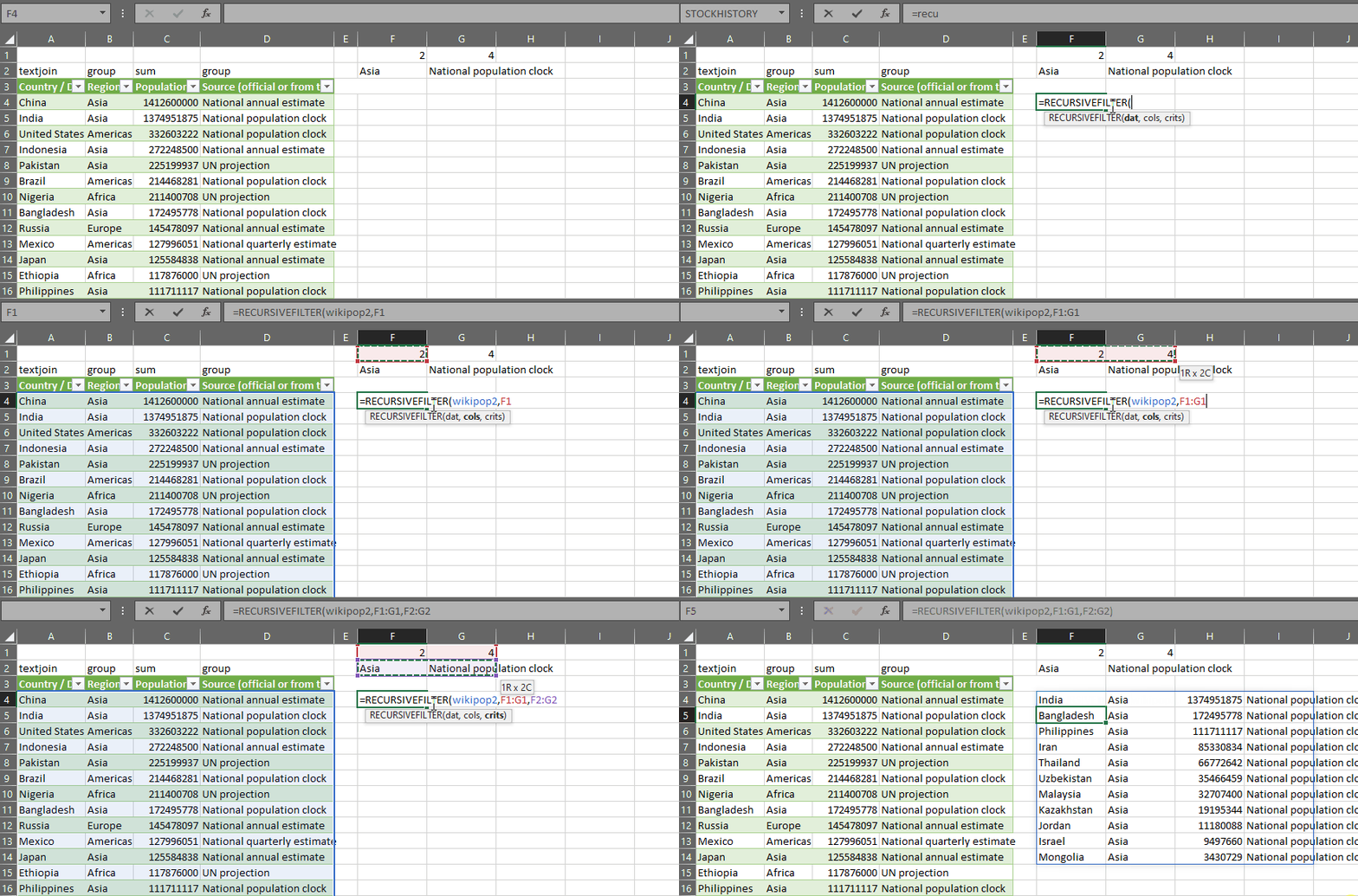
Here’s an example showing RECURSIVEFILTER in action.

This filter’s columns 2 and 4 (region and source) by the values “Asia” and “National population clock”.

So there you have it, now you can use Excel’s FILTER function with dynamic lists of filters.

There are some limitations at the moment which I might improve in the future:

1. The filters are always AND – RECURSIVEFILTER doesn’t support OR currently
2. There can only be one filter per column
3. We can only filter using the = operator
4. The list of columns is a list of column numbers – you can’t pass a list of column names currently

This list of limitations might seem to make the function not very useful, but it fits the purpose I originally created it for.

The reason I created RECURSIVEFILTER wasn’t so I could use it in the worksheet on its own. It was actually so I could pass it into a more useful LAMBDA called GROUPAGGREGATE, which is the subject of another post.