excel-lambda-NONEMPTYROWS: Filter Out Rows With Empty Cells

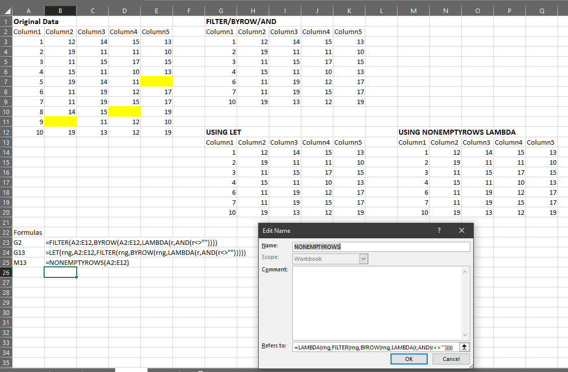
If you want to quickly get all rows which don’t have any blanks in any columns, you can combine FILTER, BYROW and AND, like this:

=FILTER(range,BYROW(range,LAMBDA(r,AND(r<>””))))

Here, I’ve defined a LAMBDA function, which is really just a way of applying some logic (in the second parameter) to some data (in the first parameter). I have “r” as the name for my data.

By passing that LAMBDA as the second parameter of BYROW, I’m telling Excel that “r” represents a row of “range” and that I want the function AND(r <> “”) to be applied to that row.

That AND function will check if each column in the row is not empty. If they’re all not empty, it will be TRUE. If any column in that row is empty, it will be FALSE. So, BYROW does this for each row in the range and returns a 1-column array of TRUE/FALSE that has the same number of rows as “range”. I then use that TRUE/FALSE array as the “include” parameter of the FILTER function.

So, for the data in “range”, check if the cells in each row are all non-empty. If they are, then include the row. Otherwise, exclude it.

Where I’ve written “range” above, you would need to select exactly the same cells in both places. So, it may be easier to use LET to only have to select those cells once. Like this:

=LET(rng,A2:E12,FILTER(rng,BYROW(rng,LAMBDA(r,AND(r<>””)))))

LET allows you to give names to functions or ranges so you can re-use the name in several places in a formula instead of having to enter that function or range multiple times.

Further to all this, I think I’ll probably use this kind of thing again, so I can wrap the entire function in a LAMBDA function of its own and define it in the Name Manager. I’ve called it NONEMPTYROWS.

This is the LAMBDA called NONEMPTYROWS:

=LAMBDA(rng,FILTER(rng,BYROW(rng,LAMBDA(r,AND(r<>””)))))

If you wanted to switch this around to return only those rows that have a blank in any column, you would replace the AND(r<>””) with OR(r=””).